Digital advertising has a fundamental incrementality measurement problem. When sales increase after a campaign launch, we can’t separate the impact of our ads from everything else happening in the market – seasonality, competitor actions, economic shifts, or simply organic growth. Traditional attribution methods are failing as cookie deprecation accelerates and cross-device tracking becomes impossible.
The GeoLift framework provides a solution: a rigorous incrementality testing approach to isolating the true incremental impact of advertising spend using geo testing marketing experiments. This methodology enables causal impact analysis that proves what revenue your ads actually created.

What is GEO Lift?
GeoLift is a causal impact analysis methodology that measures advertising effectiveness through geo testing marketing – dividing geography instead of users for incrementality measurement.
The principle is straightforward: select two statistically similar markets, cities, regions, or any definable geography. Run your advertising campaign in one market (the Test) while withholding it from the other (the Control). By comparing their performance during the campaign period, you isolate the incremental revenue generated specifically by your advertising. The selection isn’t manual – an algorithm analyzes historical data to identify pairs that move together with high correlation, ensuring mathematical rather than intuitive similarity.
As Google researchers Jon Vaver and Jim Koehler define it: “Geo experiments are randomized field tests that manipulate advertising spend across geographic regions to estimate incremental ad impact on business outcomes.”
The method works because geographic separation is clean and unambiguous. A person is physically present in one location or another. No cross-contamination, no cookie deletion issues, no cross-device tracking problems. If Portland and Austin historically move in lockstep – when one grows 5%, the other grows 5% – then any divergence during a test period where only Portland receives advertising can be attributed to that advertising with mathematical confidence.
This isn’t new. Google has published research on geo experimentation, and sophisticated retailers have used regional testing for decades. What’s changed is accessibility. The statistical tools required – Bayesian time series models, correlation analysis, power calculations – are now available as open-source Python libraries. What once required a team of PhDs can now be implemented by any competent data analyst with the right framework.
Why This Matters
The value of GEO Lift comes down to three outcomes that directly impact business decisions.
Clean incrementality measurement. Most advertising metrics are inflated because they count baseline sales – purchases that would have happened even without ads. A customer searching for your brand name was probably going to buy anyway. GeoLift incrementality testing isolates only the additional revenue created by your campaign, giving you true incremental Return on Ad Spend (iROAS). This is what your CFO actually cares about: how many dollars of new revenue did each dollar of ad spend generate?
Statistical confidence. The framework produces a P-Value for every test, quantifying the probability that your results are due to random chance rather than your advertising. When you present results with 95% confidence (P < 0.05), you’re telling finance there’s less than a 5% chance this outcome happened by accident. That level of rigor transforms marketing from a cost center with vague ROI claims into a growth driver with proven returns.
Better scaling decisions. Once you’ve proven that a channel delivers 4.0 iROAS in one market with statistical significance, you have a defendable basis to increase budget nationally. Conversely, if a test shows no significant lift, you can cut spending before wasting money at scale. You’re measuring what matters: did this advertising create revenue that wouldn’t have existed otherwise?
Why Most GEO Tests Fail
Running a geo lift test sounds straightforward in theory, but the majority of attempts produce inconclusive or misleading results. The problem isn’t the concept – it’s the execution. Most teams skip critical validation steps or make assumptions that invalidate their conclusions before the test even begins.
Understanding these common pitfalls is essential for successful incrementality testing in marketing – later in this article, I’ll walk through the specific configurations and validation steps needed to avoid each one.
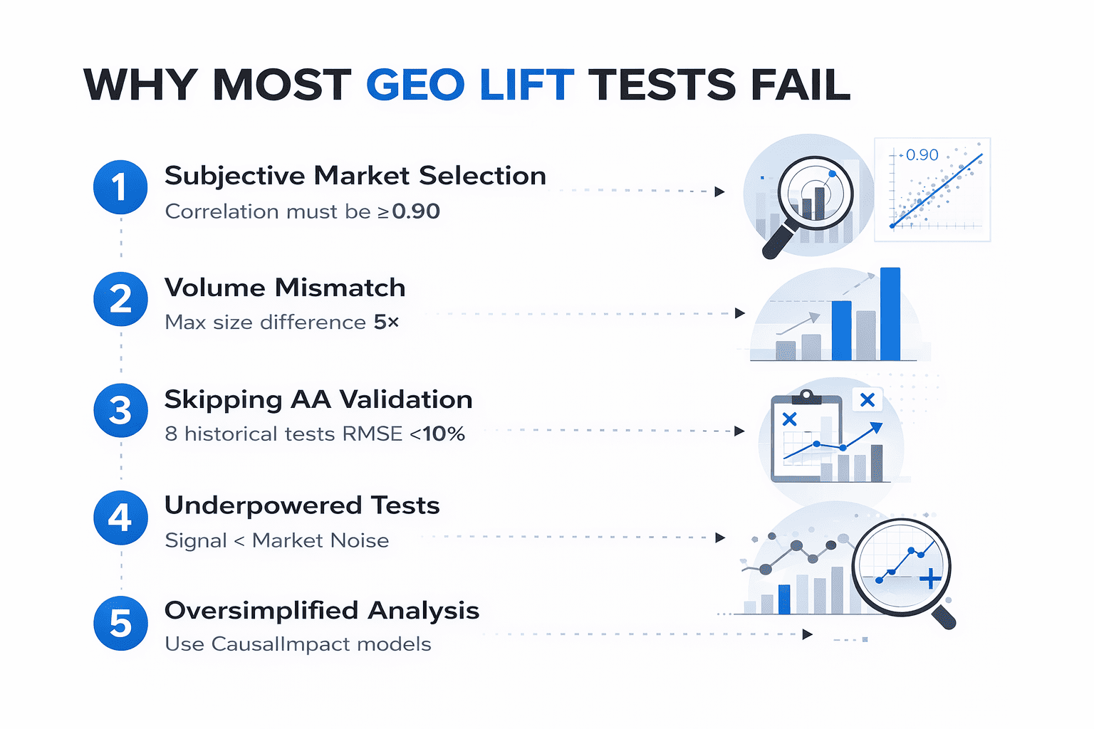
Choosing Markets Subjectively
A marketing director looks at a map and decides that Charlotte and Nashville should be comparable test markets because they’re both mid-sized Southern cities with similar demographics. This approach fails because subjective similarity doesn’t guarantee statistical similarity.
Charlotte might be heavily influenced by financial services employment, while Nashville’s economy runs on healthcare and tourism. Their revenue patterns could be completely uncorrelated despite appearing similar on paper. If two markets don’t move together historically – if one consistently trends upward while the other fluctuates unpredictably – then any difference you observe during a test period is just as likely to be their natural divergence as it is to be your advertising impact.
The framework addresses this by calculating Pearson correlation across the entire historical dataset. Only pairs with correlation above 0.90 qualify for consideration, and ideally you want 0.95 or higher.
Volume Mismatch Between Test and Control Regions
Comparing New York to Albany might show high correlation in percentage terms, but the absolute scale difference makes prediction unstable. New York’s weekly revenue fluctuations in dollar terms could exceed Albany’s entire weekly revenue.
When markets operate at fundamentally different scales, they respond differently to the same external factors. A 2% market-wide shift might be imperceptible noise in the larger market but a significant signal in the smaller one.
The framework enforces volume parity by rejecting any pair where one market is more than five times the size of the other. This keeps comparisons meaningful – the markets need to be operating at similar enough scale that they experience comparable variance.
Skipping Historical Validation (AA Tests)
Finding a pair with 0.92 correlation feels like success, so the natural impulse is to immediately launch the test. But correlation can be coincidental or time-period specific. Two markets might correlate beautifully from January to June, then completely diverge in July due to local factors that don’t show up in aggregate correlation statistics.
The AA validation stage runs eight separate simulations using historical data – periods where no advertising was running. If the Control market can consistently predict the Test market with less than 10% error across all eight periods, you have proof of reliability. If it can’t, the pair gets rejected before you spend a dollar.
Underpowered Tests and Budget Miscalculation
Every market has natural volatility – weekly revenue bounces around even when nothing is happening. If that natural noise is $8,000 per week and you launch a campaign expecting to generate $3,000 in incremental revenue, the algorithm will never be able to distinguish your signal from the background fluctuation.
You’ll finish the test, run the analysis, and get a result that says “not significant” even if your advertising actually worked. The test was underpowered from the start.
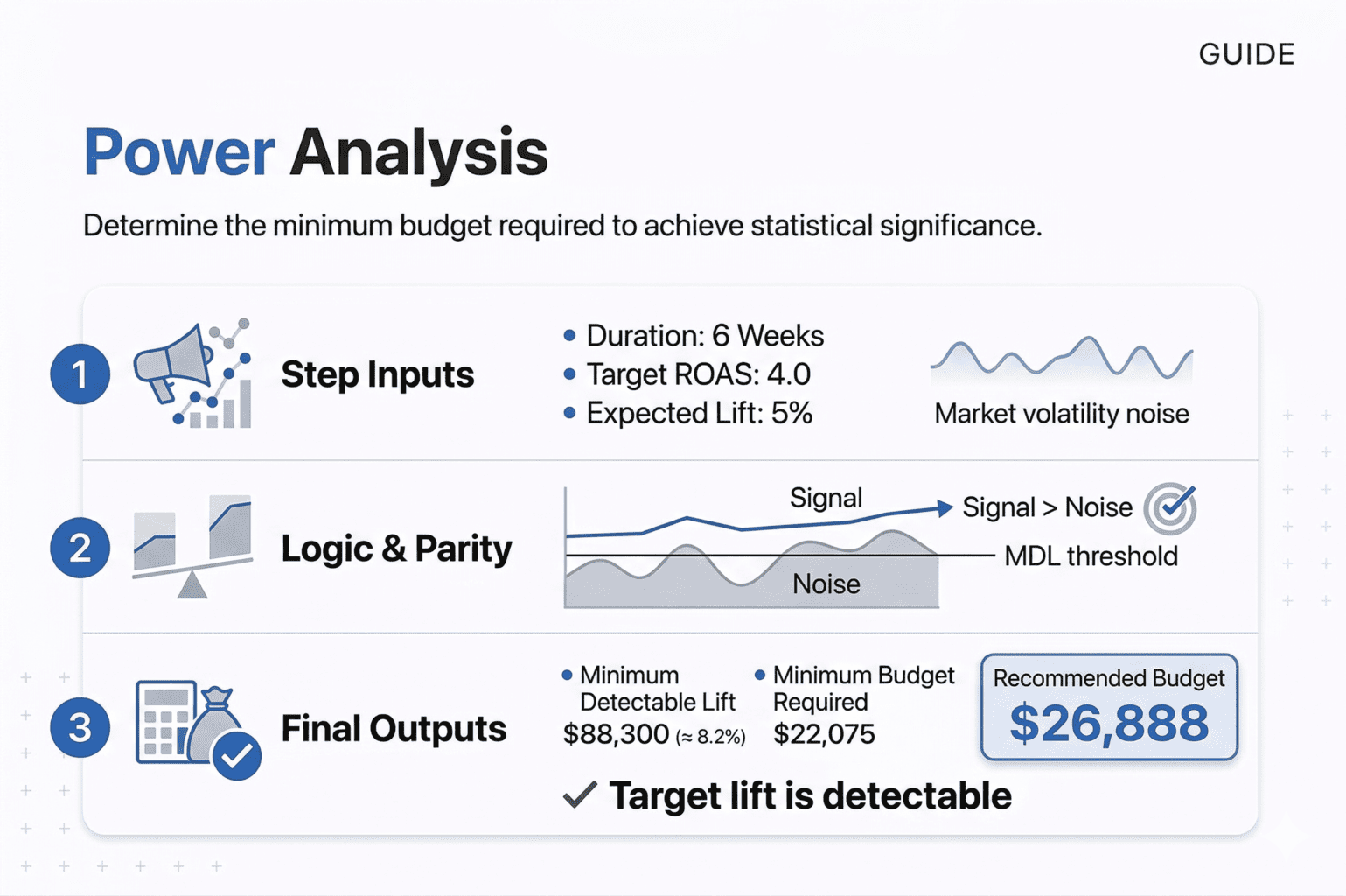
Power analysis solves this by calculating the Minimum Detectable Lift before you begin. It measures the market’s volatility, accounts for your test duration, and tells you the exact revenue threshold needed for statistical significance. If the minimum budget exceeds what you’re willing to spend, you either extend the test duration, pick a less volatile market, or acknowledge that the test isn’t feasible.
Oversimplified Analysis Without Causal Models
The most basic approach is to compare revenue before and after the campaign – if it went up, the ads worked, right? This completely ignores everything else happening in the market. Seasonal trends, competitor actions, economic conditions, even weather patterns affect sales.
Slightly more sophisticated teams use difference-in-differences, comparing the change in Test versus Control. This is better, but it still assumes linear trends and equal external effects across markets.
The framework uses Bayesian Structural Time Series modeling through the CausalImpact library. This builds a counterfactual prediction – a probabilistic model of what would have happened in the Test market if advertising had never run, based on the Control market’s behavior and the historical relationship between them. The difference between this counterfactual and actual results is the true incremental impact.
The GEO Lift Framework: Step-by-Step Implementation
The framework consists of five sequential stages, each with specific configuration parameters and validation checks. These aren’t optional steps – skipping any one of them will compromise the reliability of your results. I’ll walk through each stage with the exact settings and logic behind them.
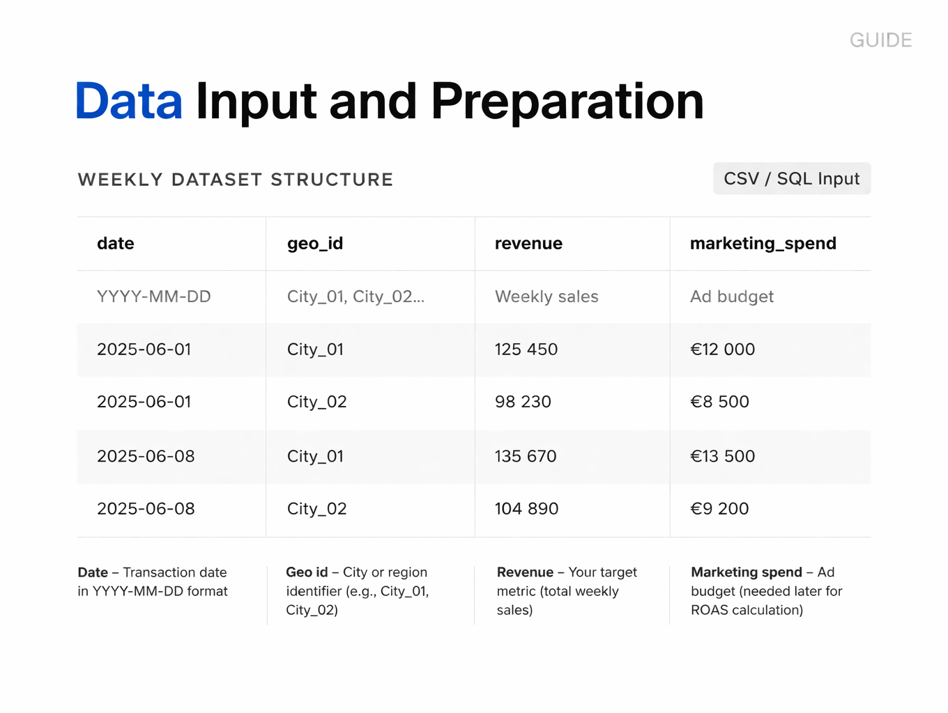
Step 1 – Data Input and Preparation
The quality of your input data determines everything downstream. The algorithm needs clean, structured historical data to learn how each market behaves over time – its seasonal patterns, response to external events, and natural volatility.
Required Data Structure
Your input file should be a CSV with four columns:
- Date – Transaction date in YYYY-MM-DD format
- Geo id – City or region identifier (e.g., City_01, City_02)
- Revenue – Your target metric (total weekly sales)
- Marketing spend – Ad budget (needed later for ROAS calculation)
Why Weekly Granularity Is Critical
This is where most people make their first mistake. Raw transactional data comes in daily, and the instinct is to use it directly because it feels like more information. Don’t.
Daily data is too noisy. Monday sales are always lower than Friday sales. A single large order on Tuesday creates a spike that looks significant but means nothing. If you try to find correlation between cities at the daily level, random day-of-week effects will overwhelm the actual market patterns you’re trying to detect.
Aggregate everything to weekly buckets. Sum revenue from Monday through Sunday for each city. This smooths out the day-of-week noise while preserving real trends. Weekly granularity also aligns with how most campaigns are planned and budgeted, making the results more actionable.
Minimum Historical Data Requirements
You need a minimum of 12 months of continuous historical data before your test period. This isn’t arbitrary – the algorithm needs to observe each market through a full seasonal cycle. Holiday patterns, summer slowdowns, back-to-school spikes – all of these need to be captured in the training data.
Less than 12 months and the model won’t have learned enough about seasonality. It might see a December spike in the Test market and incorrectly attribute it to your advertising when it’s actually just Christmas shopping that happens every year.
Step 2 – Market Selection Algorithm
This stage identifies pairs of markets that move together historically. The algorithm evaluates every possible city combination and filters them through three sequential tests. Only pairs that pass all three make it to the candidate list.
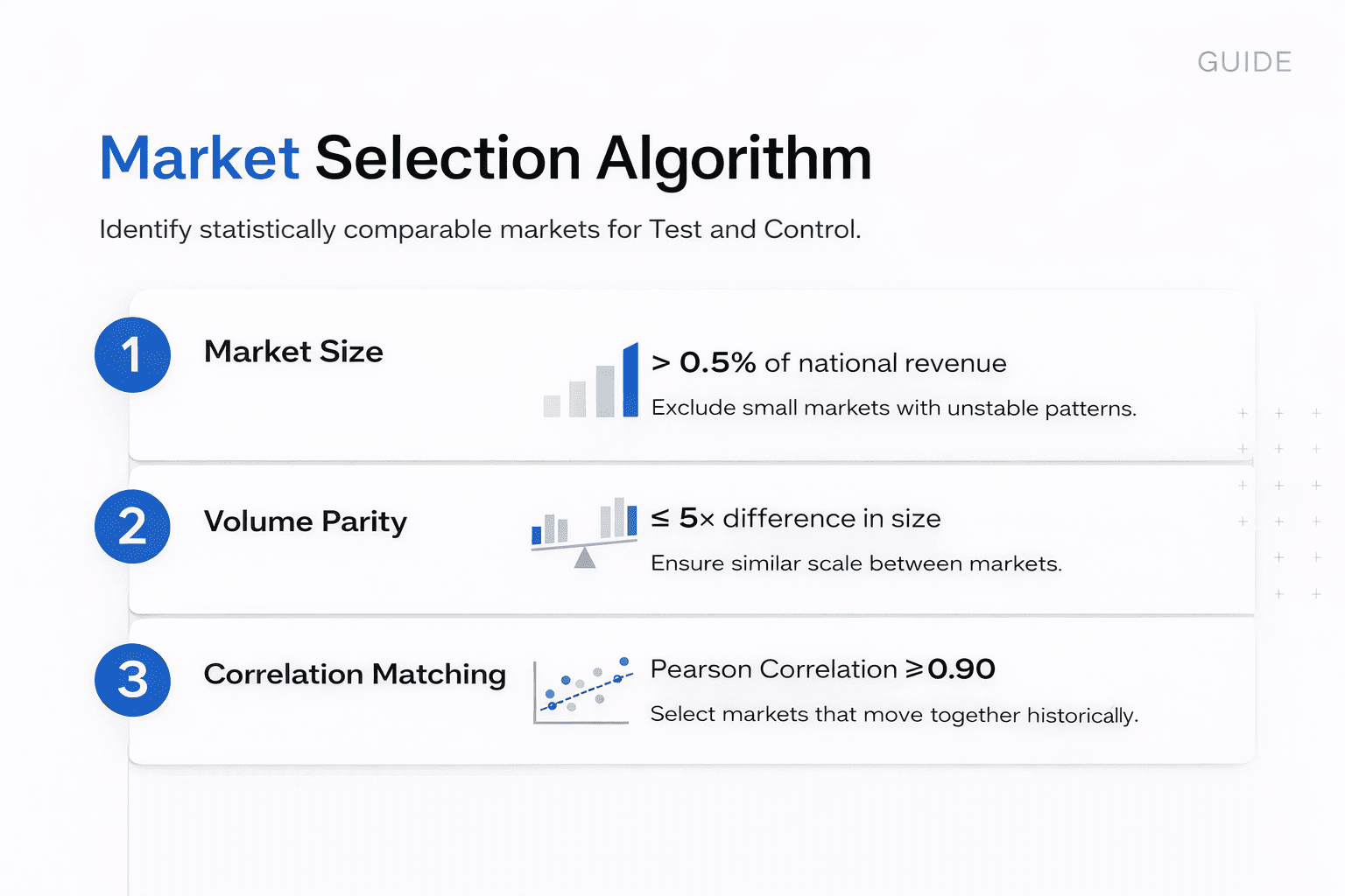
Minimum Market Share Filter
The first filter removes markets that are too small to be statistically reliable. Any city contributing less than 0.5% of total national revenue gets excluded automatically.
Why this threshold? Small markets are inherently volatile. If a town generates $2,000 in weekly revenue, one customer buying an extra $400 creates a 20% spike. That’s not a trend – it’s noise. The algorithm would see these random fluctuations and mistake them for correlation with other markets. By enforcing a minimum size, we ensure every market in consideration has enough transaction volume to exhibit stable patterns.
Volume Parity Threshold
The second filter prevents “apples to oranges” comparisons. Even if two markets are correlated, they need to operate at similar scale for the comparison to be meaningful.
The parameter is set to 0.8, which translates to a maximum 5x size difference. The smaller market must be at least 20% the size of the larger one. For example, comparing a $100,000/week city to a $150,000/week city passes (difference = 0.33). Comparing a $100,000/week city to a $600,000/week city fails (difference = 0.83).
Why does scale matter? Because markets of different sizes respond differently to the same external shocks. A competitor opening a new location might be imperceptible noise in New York but a major market shift in a smaller city. Volume parity ensures comparable sensitivity to external factors.
Correlation Threshold and Market Matching Output
This is the core matching algorithm. The script calculates Pearson correlation between every qualifying pair using their entire historical revenue series.
Correlation measures synchronization: when Market A grows 5%, does Market B also grow approximately 5%? When Market A dips in February, does Market B follow the same pattern? A correlation of 1.0 would be a perfect match (impossible in reality). A correlation of 0.0 means no relationship at all.
The threshold is set at 0.80, meaning 80% of the variance in one market needs to be explained by the other. In practice, you should be aiming for pairs above 0.90. Anything below 0.80 means the markets are too dissimilar—their behaviors diverge too often to make reliable predictions.
Algorithm Output
The script iterates through every possible combination (City_01 vs City_02, City_01 vs City_03, etc.) and keeps only pairs passing all three filters. The results are saved to a CSV file ranked by correlation score, highest to lowest.
What you’re looking at in that output file is a list of mathematically validated market pairs. These aren’t subjective guesses – they’re cities that have proven they move together over months of historical data, operate at comparable scale, and generate enough volume to be statistically stable.
Step 3 – AA Test Validation (Historical Placebo Testing)
Finding a pair with high correlation is necessary but not sufficient. Correlation can be accidental, or it might only hold during certain periods. Before you commit real advertising budget, you need proof that the Control market can actually predict the Test market accurately.
This is where AA validation comes in – it’s a stress test using historical data.
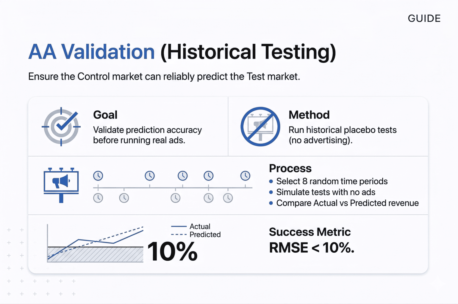
The Historical Placebo Concept
The algorithm goes back in time to periods when no advertising was running in either market. It pretends a campaign started on a specific historical date and uses the Control market to predict what should have happened in the Test market during those weeks. Since there were no actual ads, the prediction and reality should match almost perfectly. Any discrepancy reveals that the pair is unreliable.
If the algorithm detects “ghost lift” – a significant difference between prediction and actual performance when no marketing was happening – it means the pair isn’t stable enough. Random divergence between the markets will be mistaken for advertising impact during a real test.
Why Multiple Validation Windows Matter
Key Configuration: NUM_SHIFTS = 8
The framework doesn’t just test once. It runs eight separate simulations, each starting at a different point in your historical data, each lasting four weeks (typical campaign duration).
Why multiple simulations? Because a pair might correlate perfectly in January but diverge badly in July. Maybe one market has a local event that affects summer sales. Maybe tourist patterns differ. Testing across eight different time windows proves the pair is stable across seasons, holidays, and varying market conditions.
RMSE Threshold and Pass/Fail Logic
Success Metric: RMSE < 10%
The pass/fail decision is based on Root Mean Square Error (RMSE), calculated using numpy. This measures the average prediction error as a percentage of actual revenue.
Here’s what the numbers mean:
- RMSE of 5% = the Control market predicts the Test market with 95% accuracy
- RMSE of 10% = 90% accuracy (our threshold)
- RMSE of 20% = 80% accuracy (too volatile, pair rejected)
Why is 10% the cutoff? Because most advertising campaigns generate 5-10% incremental lift. If your baseline prediction error is already 15%, you’ll never be able to see the advertising signal – it will be buried in the natural noise between the two markets. The test becomes unreadable.
Validation Output
Each pair receives a status: PASSED or FAILED. Only passed pairs move forward to the testing stage. Failed pairs get discarded regardless of their correlation score. This single validation step eliminates the majority of false positives that would otherwise waste budget on unreliable experiments.
Step 4 – Power Analysis and Budget Calculation
You’ve identified a validated pair. Now comes a critical question: how much money do you need to spend for the test to produce a conclusive result?
This isn’t about what you can afford or what feels right. It’s a mathematical calculation that determines whether your test will be able to detect the advertising impact at all.
Why Budget Size Matters Statistically
Every market has natural volatility. Sales go up and down week to week even when absolutely nothing changes in your marketing. This random fluctuation is noise. Your advertising creates a signal – an increase in revenue above what would have happened naturally.
For the test to work, your signal needs to be larger than the noise. If you generate $5,000 in incremental revenue but the market naturally fluctuates by ±$8,000, the algorithm can’t tell the difference between “the ads worked” and “it was just a good week.”
How the Minimum Detectable Lift (MDL) Is Calculated
The framework uses scipy.stats for statistical thresholds and numpy for volatility calculations. Here’s the process:
First, the script measures your Test market’s historical weekly revenue standard deviation. If a market’s weekly revenue typically fluctuates by $8,000, that’s your weekly noise level.
Next, it scales this over your test duration using the square root rule: Total Noise = Weekly Volatility × √(Number of Weeks). So $8,000 weekly volatility over 6 weeks becomes $8,000 × √6 = $19,596, not $48,000. Random fluctuations partially cancel out over time.
Then it applies your confidence threshold. The CONFIDENCE_LEVEL parameter (typically 0.90 for 90% confidence) converts to a Z-score of 1.28 using scipy.stats. This represents how many standard deviations away from normal the result needs to be for us to believe it’s real.
Required Budget for Statistical Significance
Using our example: $19,596 × 1.28 = $25,083. This is the minimum incremental revenue your campaign must generate for statistical significance.
Finally, convert to required budget using your TARGET_ROAS parameter: Minimum Budget = MDL / Target ROAS. If MDL is $25,083 and you expect 4.0 ROAS, you must spend at least $6,271.
Feasibility Check: Is the Test Statistically Possible?
The script compares your expected lift against the MDL. If you’re expecting 5% growth but the MDL requires 8% to be detectable, it warns you: “Your target lift is below the noise level.”
You have three options: increase budget, extend test duration, or choose a less volatile market. What you cannot do is proceed and expect conclusive results.
This calculation prevents the most common waste in testing – spending $30,000 on experiments that required $50,000 minimum to be readable, getting “not significant” results, and incorrectly concluding the channel doesn’t work.
Step 5 – Causal Impact Analysis with Bayesian Structural Time Series
The test is complete. You’ve spent the budget, the campaign has run, and now you need the answer: did the advertising actually work?
This is where the framework moves from correlation to causation. Simple before-and-after comparisons are worthless because they attribute everything to your ads – seasonal trends, competitor mistakes, economic changes, all of it. We need to isolate only the revenue that wouldn’t have existed without your advertising.

CausalImpact and Bayesian Structural Time Series Model
The causal impact analysis uses the causalimpact library, which implements Bayesian Structural Time Series modeling. This was originally developed by Google in R and later ported to Python. The concept is elegant: build a prediction of what should have happened in the Test market based on the Control market’s behavior, then compare that prediction to reality.
Defining the Pre-Period and Test Period
Two parameters are critical: TEST_START_DATE and TEST_END_DATE. These define the exact boundaries of your campaign period. One day of overlap between training and testing will corrupt the model, so precision matters.
The algorithm splits your data into two periods:
- Pre-period (training): All historical data before the test started, where it learns the relationship between Test and Control
- Post-period (testing): The weeks when advertising was running, where it measures the impact
How the Counterfactual Prediction Is Built
During the pre-period, the model learns how the Test and Control markets move together. It doesn’t just look at correlation – it builds a probabilistic model of their relationship that accounts for trends, seasonality, and varying external conditions.
Then it projects this learned relationship forward into the test period and asks: “What would have happened in the Test market if we had never launched ads?” This projection creates the counterfactual baseline – the blue dotted line you see on CausalImpact charts.
The black line represents what actually happened. The gap between them is your answer.
Core GEO Lift Output Metrics
The analysis produces three outputs:
- Incremental Revenue is the difference between the actual revenue (black line) and the predicted baseline (blue line), summed across all test weeks. This is the only revenue number that counts. Total revenue is meaningless because it includes all the sales that would have happened anyway. Incremental revenue is what your advertising created.
- iROAS (Incremental Return on Ad Spend) divides incremental revenue by your ad spend. If you spent $10,000 and generated $42,000 in incremental revenue, your iROAS is 4.2. Every dollar spent created $4.20 in new revenue. This is fundamentally different from platform-reported ROAS, which inflates results by counting baseline sales.
- P-Value is your confidence check. It represents the probability that the observed lift could have happened by random chance. A P-Value of 0.03 means there’s only a 3% chance this was luck – you’re 97% confident the ads caused the lift. A P-Value of 0.18 means there’s an 18% chance it was random market noise – not conclusive enough to claim success.
Significance Threshold and Result Interpretation
The standard cutoff is P-Value < 0.10 for 90% confidence (matching your CONFIDENCE_LEVEL parameter from power analysis). Some businesses use 0.05 for 95% confidence. Anything above these thresholds means “not significant” – you cannot conclusively say the advertising drove the result.
This is where underpowered tests reveal themselves. If you didn’t spend enough budget (ignored the power analysis), you’ll see incremental revenue but a high P-Value. The algorithm is saying “yes, there’s a difference, but it’s not large enough relative to the noise for me to be confident it’s real.”
Visualizing Incrementality Results
The framework generates a chart using matplotlib that shows three panels: the original data with actual vs predicted, the pointwise contribution (lift over time), and the cumulative effect. This visualization makes the result immediately clear – you can see exactly when the lift occurred and how it accumulated.
When you present this to stakeholders, you’re showing them the counterfactual world alongside reality, with statistical confidence intervals. It’s far more convincing than saying “sales went up 12%.”
Technical Implementation Notes
The time series needs to be explicitly set to weekly frequency using df.asfreq(‘W-MON’) or the library will misinterpret the data structure. Missing weeks should be filled with zeros to prevent crashes. And you’ll likely need to suppress FutureWarning messages because CausalImpact hasn’t been updated for the latest pandas versions – these warnings don’t affect functionality.
The output is clean: you get incremental revenue, iROAS, and P-Value. If P < 0.10 and iROAS exceeds your target, the test succeeded. If P > 0.10, the result is inconclusive regardless of the revenue numbers. And if iROAS is below target even with significance, the channel is unprofitable at scale.
This final stage answers the only question that matters: did this advertising create revenue that justifies the spend, and can we prove it mathematically?
GEO Lift Limitations: When the Framework Does Not Work
GEO Lift is a powerful framework, but it’s not a universal solution. There are structural constraints and specific scenarios where the methodology simply breaks down. Understanding these limitations prevents wasted effort on tests that are mathematically impossible to execute.
No Geo Holdout → No Incrementality Measurement
If you want to run advertising across the entire country simultaneously and measure its impact, GEO Lift cannot help you. The methodology requires a Control market – a clean geographic area with zero advertising exposure. Without it, there’s no baseline for comparison.
Comparing “the country this month” to “the country last month” doesn’t work because it ignores seasonality, competitor actions, economic shifts, and every other external factor. The algorithm needs spatial separation, not just temporal separation. If you can’t hold out at least 10-20% of your geography as a control group, the test is impossible.
Low Budget vs High Market Volatility
You cannot test micro-budgets in high-volume markets. If your company generates millions in revenue and you want to test a $1,000 campaign, the signal will be invisible against market volatility.
The Power Analysis script calculates Minimum Detectable Lift based on natural market fluctuations. If that natural noise is $8,000 per week and your expected incremental revenue is $2,000, the result will always be “not significant” – not because the ads didn’t work, but because the test was underpowered from the start. You’re trying to hear a whisper at a rock concert.
Not Suitable for Low-Volume or Niche Businesses
B2B sales, luxury yachts, or hyper-niche e-commerce with five orders per week are poor fits for this framework. The methodology requires frequent, stable transactions.
The algorithm aggregates data weekly and filters out markets below minimum volume thresholds. When your sales chart looks like 0, 1, 0, 2, 0, 3 – it’s not a trend, it’s randomness. Finding correlation above 0.80 on this kind of data is impossible. The matching algorithm will fail because there’s no stable pattern to match.
This tool works for mass market retail, FMCG, or e-commerce with consistent daily transactions. Infrequent, high-value sales don’t generate the data density required.
Channels Without Geo Targeting Break the Model
If you want to test influencer marketing, organic social, SEO, or PR, you likely cannot enforce clean geographic boundaries. You can’t tell a YouTube creator “only show this video to people in Portland.” You can’t prevent someone in the Control city from searching for your brand and finding your newly optimized content.
The framework requires channels with strict geo-targeting capabilities – Google Ads, Facebook Ads, regional TV, geo-fenced digital outdoor. Any “leakage” where Control market residents get exposed to your advertising contaminates the test. The independence assumption breaks down and results become unreliable.
Speed: Not for Quick Iterations
GEO Lift is not a tactical testing tool. The minimum test duration is 4-6 weeks because the algorithm needs time to accumulate statistical significance. You cannot “quickly test this creative over the weekend.”
This is a strategic instrument for validating channels, informing annual budgets, or proving incrementality to finance teams. If you need to test button colors, landing page variants, or ad copy, use platform-level A/B tests. Those run in days with clear results. Geographic experiments run in months.
Multichannel Testing
If you simultaneously launch a new website, change pricing, and start TikTok advertising in the Test market, the algorithm will show lift but cannot tell you which intervention caused it.
GEO Lift measures aggregate impact. The code will report that revenue increased by 15%, but it has no way to decompose that into “8% from pricing, 5% from TikTok, 2% from the website.” You’ll know something worked, but not what.
The rule is strict: one variable at a time. Change only the marketing intervention you’re testing. Hold everything else constant. Otherwise you’re running an uninterpretable experiment.
What does Geo Lift incrementality testing give
GeoLift incrementality testing solves digital advertising’s core incrementality measurement problem: proving what revenue your ads actually created versus what would have happened anyway through rigorous causal impact analysis.
The framework requires discipline – clean data, statistical validation, proper budgeting, and causal modeling – but that rigor is what makes it reliable. At the end, you get three numbers: incremental revenue, iROAS, and P-Value. Not estimates. Not attribution models. Mathematical proof of impact with quantified confidence.
The limitations are real. You need geographic targeting capability, sufficient transaction volume, adequate budget, and the discipline to test one variable at a time. This isn’t for quick tests – it’s for strategic decisions about channel validation and budget allocation. But if your situation fits, this framework gives you what cookie-based attribution never could: the ability to prove exactly how much incremental revenue each advertising dollar generated. The tools are accessible. The methodology is proven. The question is whether you’re ready to measure what actually matters.